Hill – Mankiw 9th Edn Chapter 20 – Income Inequality and Poverty
Mankiw, N. G. (2021) Principles of microeconomics (9th ed.)
Principles of economics (9th ed.)
Mason, OH: South-Western Cengage Learning.
Rod Hill
University of New Brunswick, Saint John campus
Saint John, New Brunswick, Canada
email: rhill@unb.ca
Chapter 20 – Income Inequality and Poverty
Here are some things to consider when reading this chapter.
- Economists’ views on income redistribution
Mankiw writes: “many economists – though not all – believe that the government should redistribute income to achieve greater equality”. He adds that policies to redistribute income involve a trade-off because they distort incentives, alter behavior, and make “the allocation of resources less efficient” (p. 398).
A 2020 survey of members of the American Economic Association asked for their views about this normative statement: “The distribution of income in the US should be more equal.” (For the distinction between positive and normative statements, see Mankiw’s explanation on page 26.)
Of those who responded, 14 percent disagreed with the statement; 65 percent agreed without any provisos; 21 percent agreed with provisos. In earlier surveys in 1990 and in 2000, 32 percent disagreed that the income distribution should be more equal (Geide-Stevenson and La Parra-Perez 2024, p. 464).
One could disagree with the statement for three reasons: (i) judging current income inequality to be ethically acceptable, so further redistributive measures are not needed; (ii) judging that less inequality would be ethically desirable, but the cost of doing so is too great; or (iii) taking the philosophical position that governments should not redistribute market incomes, no matter what they are.
Relevant to this last possibility, the survey also reported opinions about another normative statement: “Redistribution of income is a legitimate role for the US government”. In 2020, 13.7 percent disagreed with this, down from a high of 25.5 percent in 1990 (p. 465). Respondents who think government shouldn’t redistribute market incomes are ‘economic libertarians’ who might subscribe to the ideas of libertarian philosopher Robert Nozick, which Mankiw summarizes.
Such libertarians say that if the processes that produce economic outcomes are fair, then the outcome is fair. Mankiw (p.409) quotes Nozick: “What each person gets, he gets from others who give to him in exchange for something, or as a gift. In a free society, diverse persons control different resources, and new holdings arise out of the voluntary exchanges and actions of persons.”
In such a libertarian society, there would be no social insurance such as universal old-age pensions, unemployment insurance, welfare assistance to those with minimal incomes. These would require involuntary redistribution through taxation by government, violating people’s property rights over their justly-earned market incomes. Those who can’t sell their labour for enough to exist, would have to rely on the charity of family, friends, or charitable organizations.
However, the libertarian emphasis on voluntary exchanges ignores the power relationships within which those exchanges take place. The Commentaries on Chapters 6 and 18 explain that employers typically have some monopsony power; the previous two Commentaries discuss how those exchanges also take place within a legal and regulatory environment that some economic actors have had the power to shape to their advantage. Given this, has the resulting distribution of income been attained fairly?
Note that the marginal productivity theory of factor prices set out in Chapters 18 and 19 says nothing about whether, for example, wages are what people deserve. It’s not a normative theory; it’s a positive theory that might be used for explanatory or predictive purposes. When the theory was originally developed in the late 19th century, some did claim that the theory described actual markets and that paying factors the value of their marginal product was equitable, making the theory normative as well. However, that position has long since been discarded in neoclassical economics (Hill and Myatt 2022, pp. 209-12). A few textbooks tell students that the theory is not normative, but most say nothing.
- Growing income inequality and its causes
(i) Growing income inequality
Mankiw’s description of increasing income inequality in the United States since 1970 includes data on the shares of total income received by people within the top 1 percent of income recipients (p. 400). The increases in these shares have contributed significantly to the increase in overall inequality.
Mankiw gives no source, but his numbers match the data used in Saez (2023) for income excluding capital gains. Saez’s paper gives a link to his spreadsheet file which contains data for income including and excluding capital gains. Including capital gains (or losses) can change a group’s income share sharply from year to year. For example, in 2021 capital gains among very high-income groups were unusually large as the stock market rebounded after the pandemic. Excluding capital gains avoids giving undue weight to these short-term fluctuations. But when looking at long-term changes in income shares, including capital gains in the measure of income is desirable because they are an important component of the incomes of high-income individuals.
Tables 20.1 and 20.2 show the changes in income shares and the percentage changes in them for both measures of income (with and without capital gains) for three groups: the top 1 percent, and the top 10th and the top 100th of the top 1 percent. Mankiw cites data for 2017, the latest available at the time he was writing, but data up to 2021 is now available.
Table 20.1: Shares of total income, including capital gains, by income group, 1970-2021
| Top | 1970 | 2017 | 2021 | Change 1970-2017 | Percent Change 1970-2017 | Change 1970- 2021 | Percent change 1970-2021 |
| 1 percent | 9.03 | 22.01 | 27.40 | 12.98 | 143.7 | 18.37 | 203.4 |
| 0.1 percent | 2.78 | 10.95 | 14.85 | 8.17 | 293.9 | 12.07 | 434.2 |
| 0.01 percent | 1.00 | 5.41 | 7.46 | 4.41 | 441.0 | 6.46 | 646.0 |
Source: author’s calculations from Saez’ data. Top 1 percent: Table A3, column P99-100: Table A3, column P99.9-100; Top 0.01 percent: Table A3, column P99.99-100.
Table 20.2: Shares of total income, excluding capital gains, by income group, 1970- 2017 and 2021
| Top | 1970 | 2017 | 2021 | Change 1970-2017 | Percent change 1970-2017 | Change 1970-2021 | Percent change 1970-2021 |
| 1 percent | 7.80 | 18.17 | 20.70 | 10.37 | 132.9 | 12.9 | 165.4 |
| 0.1 percent | 1.94 | 7.82 | 9.42 | 5.88 | 303.1 | 7.48 | 385.6 |
| 0.01 percent | 0.53 | 3.40 | 4.14 | 2.87 | 541.5 | 3.61 | 681.1 |
Source: author’s calculations from Saez’ data. Top 1 percent: Table A1, P99-100. Top 0.1 percent: Table A1, column P99.9-100; Top 0.01 percent: Table A1, column P99.99-100.
Whether for 1970-2017 or 1970-2021, both tables show that the percentage change in income share is higher the higher the income group, whether income shares are measured including or excluding capital gains. The percentage increase of the top 0.01 percent is far higher than that for the top 0.1 percent, which, in turn, is higher than that for the top 1 percent as a whole. As a result, even within the top 1 percent, income inequality has increased significantly, with top income recipients enjoying a disproportionate amount of the increase in income shares received by the top 1 percent as a whole.
(ii) US income inequality in historical perspective
Estimates of income shares using income tax data have been done for the United States going back to World War I. Figure 1 shows estimates of the income share of the top decile (top 10 percent), taken from Saez (2023). Saez notes how “the shock of the war [World War II] played a key and lasting role in shaping income concentration in the United States” (p. 5). The top decile’s share remained stable until the late 1970s, when it began to increase, eventually exceeding pre-World War II values. (The series including capital gains is less smooth because of booms and busts in the stock market.)
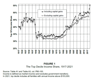
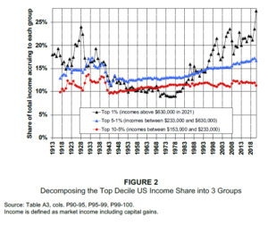
Figure 2 divides the top decile into three parts to show that the greatest variability in income shares has been experienced by the top 1 percent. The next 4 percent and the bottom half of the top decile experienced much smaller income share declines during World War II than the top 1 percent. Since the 1970s, the income share of the top 1 percent has increased sharply, the share of the next 4 percent has increased, but more modestly, and the bottom half of the top decile has seen virtually no increase in its share.
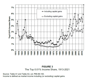
Saez’s Figure 3 shows estimates of the income shares of the top 0.01 percent – the top 1/100th of the top 1 percent. In percentage terms, the decline in its income shares during World War II and after is much greater than that experienced by the top 1 percent as a whole. Since the 1970s, its income share has increased sharply.
(iv) US income inequality in international comparison
Mankiw’s Figure 1 compares inequality across countries using the ratio of the incomes of the highest-income quintile to the incomes of the lowest-income quintile. However, it’s not clear, even from the original source, how income is measured.
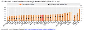
Figure 4 compares income inequality between countries in two ways (OECD 2024, p. 87). The first is the ratio of the disposable (or after-tax) incomes of the top 10 percent of the income distribution to the disposable incomes of the bottom 10 percent. Disposable income is market income plus government cash transfers minus income taxes paid. If we’re interested in the incomes available to households for their use, disposable income, appropriately adjusted for family size, is the best measure.
The second inequality measure is the Gini coefficient, which summarizes income inequality in a country using data on the entire income distribution. It can take values from 0 to 1, where higher values denote greater inequality.
As the Figure shows, by both measures the United States has the greatest income inequality among the high-income countries. The decile ratio of 17.7 is almost twice that of the OECD member country average of 8.4. The US Gini coefficient of 0.395 is about 20 percent higher than the OECD average of 0.313.
Figure 4: Income Inequality across the OECD
(iv) Why has income inequality in the United States grown since the 1970s?
While Mankiw mentions Thomas Piketty and Emmanuel Saez, who have studied growing income inequality, he says nothing about why they and others think that the shares of top incomes have grown so much. He just reiterates points raised in the previous chapter: increased trade with low-wage countries and technological changes that reduced demand for unskilled labour while raising demand for skilled labour (p. 399).
Piketty and co-authors (2014, pp. 230-231) point out that these “pure market explanations cannot account for the fact that top income shares have only increased modestly in a number of advanced countries (including Japan, Germany, or France), which are also subject to the same technological forces”. They point out that changes in institutions, “defined to include labor and financial market regulations, union policies, tax policy, and more broadly social norms regarding pay disparity” could have been important in increasing income inequality.
Saez (2023, p.7) sets out other things to consider in the case of the United States:
a significant fraction of the surge in top incomes since 1970 is due to an explosion of top wages and salaries. Indeed, estimates based purely on wages and salaries show that the share of total wages and salaries earned by the top 1 percent wage income earners has jumped from 5.1 percent in 1970 to 12.4 percent in 2007.
The labor market has been creating much more inequality over the last thirty years, with the very top earners capturing a large fraction of macroeconomic productivity gains. A number of factors may help explain this increase in inequality, not only underlying technological changes but also the retreat of institutions developed during the New Deal and World War II – such as progressive tax policies, powerful unions, corporate provision of health and retirement benefits, and changing social norms regarding pay inequality. We need to decide as a society whether this increase in income inequality is efficient and acceptable and, if not, what mix of institutional and tax reforms should be developed to counter it.
Some of the institutional changes that he describes (weakened unions, reduced health and retirement benefits) facilitated the growth of profits. Many top income recipients get an important part of their income from business profits.
Growing corporate profits also benefit corporate managers, whose salaries help to account for the growing share of wage and salary income earned by the top one percent. They can bargain over their salary with Boards of Directors. As well, reductions in top marginal income tax rates increase managers’ incentives to put more effort into bargaining to increase their salaries. If social norms evolve to accept greater pay inequality, those efforts will be even more likely to be successful (at the expense of lower paid workers and of shareholders, for whom less is left over). Consistent with this bargaining story, Piketty and co-authors (2014, p. 264) report that, in the 13 countries in their sample, the lower are top marginal tax rates, the higher is the before-tax average CEO compensation, all else equal.
(v) Reducing income inequality
If Saez’s diagnosis is correct, reversing the “retreat of institutions” that he describes would reduce income inequality. That would include measures to affect the pretax distribution of income, such as facilitating the formation of labour unions, and those affecting the after-tax distribution, such as raising top marginal income tax rates.
In their book The Triumph of Injustice, Emmanuel Saez and his colleague Gabriel Zucman ask, “Has the collapse in taxes for the ultra-rich reflected what Americans as a society wanted?” (2019, p. ix). The answer is ‘no’ according to public opinion polls that show that a consistent majority of the public (60%) are bothered “a lot” by “the feeling that some wealthy people don’t pay their fair share”. A similar majority supports increasing income tax rates on high income households.
Piketty and co-authors remark that it’s unlikely that top income earners have the ability to make large changes in their work effort in response to increased top marginal income tax rates (2014, p. 267). They estimate that additional revenue could be raised if those rates were increased to about 70 percent, as long as tax-avoidance opportunities are closed beforehand. (‘Tax avoidance’ occurs if people can shift income into a less heavily taxed category, such as capital gains. This is legal as opposed to ‘tax evasion’, which is illegal. Saez and Zucman (2019, pp. 54-56) examine the distinction.)
Piketty et al. also make a case for accompanying tax changes with regulatory measures to improve corporate governance. This would enable Boards of Directors better defend the interests of shareholders against the salary demands of corporate managers.
- The trade-off between efficiency and equality
In the first of his Ten Principles set out in Chapter 1, Mankiw claims that society faces a trade-off between efficiency, “getting the maximum benefits from its scarce resources”, and equality, distributing those benefits “uniformly among society’s members”. This concept of equality seems to refer to equality of incomes, something advocated by no one. Even the most egalitarian would not see that as a desirable goal. After all, individuals and households have different needs.
Concerning the trade-off, he writes in Chapter 1: “when the government tries to cut the economic pie into more equal slices, the pie shrinks.” The explanation: “When the government redistributes income from the rich to the poor, it reduces the reward for working hard; as a result, people work less and produce fewer goods and services” (p.2). In this chapter, the explanation is again just one sentence: “Policies that penalize the successful and reward the unsuccessful reduce the incentive to succeed.” He remarks: “This is the one lesson concerning the distribution of income about which almost everyone agrees” (p. 416).
While this may sound superficially plausible, in fact, economic theory doesn’t prove the existence of this trade-off. Whether a trade-off exists is an empirical question. Yet Mankiw cites no empirical evidence for his claim. It turns out that the evidence does not support this alleged trade-off.
In 2015, the OECD published a major study, In It Together: Why Less Inequality Benefits All. The title describes the conclusion: relatively high inequality inhibits economic growth, while a variety of policies can reduce inequality while either promoting growth or not inhibiting it. High inequality leads to wasted potential and lower social mobility for disadvantaged households, who are less able to invest in good-quality education and skills development. This results in worse job prospects, less time spent employed, and increased inequality of opportunity for their children. The authors concluded that well-designed taxes and transfers to reduce inequality do not necessarily harm growth. International Monetary Fund researchers have reached similar conclusions (Ostry, Loungani and Berg, 2019).
At the beginning of his text where he sets out his first principle, “People Face Trade-Offs”, Mankiw writes: “You may have heard the old saying, ‘There ain’t no such thing as a free lunch.’ Grammar aside there is much truth to this adage” (p.2). Yet American economist Peter Lindert explicitly contradicts this. Lindert had conducted an extensive study of the relationship in OECD countries between economic growth and social transfers such as unemployment insurance, income support, pensions, public healthcare spending, and housing subsidies (Lindert 2004a). His conclusion: “[T]he social transfers that have always defined the welfare state are indeed a ‘free lunch’ in the sense that they have delivered more equality and longer life expectancy at an essentially zero cost in terms of GDP” (2004a, p. 236).
So why do textbooks like Mankiw’s assert that the trade-off is a fact? Lindert explains that the source “is ideology and a valid theory that if governments were run badly, they would drag down economic growth” (2004b, p. 7). But the evidence suggests that, on balance, governments have acted so that the net effect of taxes and transfers and social spending has not reduced growth.
- Poverty
“Poverty is measured at different income levels, but it is experienced as an exhausting piling on of problems. Poverty is chronic pain, on top of tooth rot, on top of debt collector harassment, on top of the nauseating fear of eviction. It is the suffocation of your talents and your dreams. It is death, come early and often… Far from a line, poverty is a tight knot of humiliations and agonies, and its persistence in American life should shame us.” – Matthew Desmond (2023a)
(i) Measures of poverty in the United States
The official American definition of poverty is “an absolute rather than relative standard” (p. 401). Mankiw notes that the poverty line for a family with two adults and two children was set at $24,858 in pre-tax cash income in 2017. He adds that the US median family income that year was $75,938. (This means that half of family incomes were above this value and half below it.) The poverty rate was therefore only one third of median income.
Since 2011, annual estimates of a Supplemental Poverty Measure (SPM) have been published. The SPM includes the value of non-cash benefits that low-income families get from several government programs, such as Supplemental Nutrition Assistance Program benefits and housing assistance. The thresholds in the official poverty measure don’t vary geographically, despite differences in the cost of living. The SPM adjusts for geographic differences in housing expenses, while including federal and state taxes, work expenses, and medical expenses (Shrider 2024, p.1).
In 2023, the official poverty rate was 11.1 percent – 36.8 million people. The SPM produced a poverty rate of 12.9 percent. By this measure, the child poverty rate was 13.7 percent (Shrider 2024, p.1).
Mankiw highlights the issue of in-kind transfers and tax credits as a problem in measuring the poverty rate (p. 402). His discussion implies that poverty may not be as high as the official definition finds because these things are omitted. Yet the SPM, which he fails to mention, takes these into account, while also adjusting for regional differences in living costs. The net result is a higher poverty rate than the official definition produces.
(ii) Poverty in the United States since 1959
Mankiw’s Figure 2 (p. 401) illustrates the official poverty rate since 1959. He notes that the poverty rate fell until 1973 after which the downward trend stopped. In explaining the pre-1973 decline, it is remarkable that Mankiw fails to mention President Lyndon Johnson’s ‘War on Poverty’, initiated in 1964. As Princeton sociologist Matthew Desmond (2023b) writes:
These initiatives constituted a bundle of domestic programs that included the Food Stamp Act, which made food aid permanent; the Economic Opportunity Act, which created Job Corps and Head Start; and the Social Security Amendments of 1965, which founded Medicare and Medicaid and expanded Social Security benefits. Nearly 200 pieces of legislation were signed into law in President Lyndon B. Johnson’s five years in office, a breathtaking level of activity. And the result? 10 years after the first of these programs were rolled out in 1964, the share of Americans living in poverty was half when it was in 1960.
These measures surely contributed to the increase in real incomes at the bottom of the income distribution, helping to reduce the poverty rate. During the last 50 years, real incomes at the bottom have not increased much, leaving the poverty rate stagnant. If the antipoverty policies initiated by Lyndon Johnson were also an important cause of the initial decline in poverty, the lack of political will to take further steps would contribute to the lack of progress.
Matthew Desmond considers why political will might have petered out. He writes: “Poverty persists in America because many of us benefit from it. We enjoy cheap goods and services and plump returns on our investments, even as they often require a kind of human sacrifice in the form of worker maltreatment” (2023a).
The profitable exploitation of poor people occurs in labour, housing and financial markets, where they face the market power of employers, property owners, and financial institutions. Lack of choice leaves them accepting poor bargains: low wages and precarious working conditions, high rents for substandard housing, high bank fees, and high-interest loans from predatory lending institutions. The corresponding benefits to the rest of the population include cheaper goods and services, higher property values as the poor are kept geographically concentrated and ghettoized, and financial services subsidized by fees and interest rates charged to the poor.
(iii) US poverty rates in international comparison
Mankiw does not compare poverty in the United States with that in other countries, although this information is readily available. The OECD publication, Society at a Glance (2024), defines a poverty line at 50 percent of median income, adjusted for family size.
Such a measure of relative poverty or relative deprivation “means that richer countries have higher poverty thresholds. Higher poverty thresholds in richer countries capture the notion that avoiding poverty means an ability to access the goods and services that are regarded as customary or the norm in any given country” (OECD 2024, p. 88). In short, poverty depends on individuals’ social context. (Brady (2021) makes the case for this kind of poverty measure for the United States.)
Compared with other high-income industrialized countries, the US poverty rate of 18 percent is the highest, as seen in Figure 5. At the other end of the spectrum, poverty rates of between 5 and 7 percent can be found in countries like Czechia, Finland, Iceland, Hungary and Denmark.
Figure 5: Comparative poverty rates in 2021, OECD countries
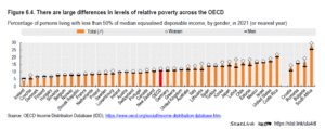
Source: Society At A Glance 2024, OECD, Figure 6.4, p. 89.
The Technical note: To compare different households, researchers adjust family income using an equivalence scale that takes family size, and possibly composition, into account. The result is a measure of “equivalized” income per person. Here, the OECD data do this by dividing household income by the square root of household size. For example, consider a household of two adults and two children whose annual income is $80,000. They would have a per-person equivalized income of $40,000 (i.e. $80,000/2). This reflects the idea that individuals in such a household would enjoy the same standard of living as a single individual with an income of $40,000.
Child poverty is a particular concern, not only for equity reasons but because of the long-term costs it can impose on them. The United Nations Children’s Fund (UNICEF) produces regular reports on child well-being, comparing countries according to various criteria. A recent report shows estimates for child poverty averaged for the years 2019-2021, as seen in Figure 6. In this case, the poverty rate is defined as the percentage of households with children w and Hans and my goodness and boss part of my photographic gem they other things there on the bed and is put on the top of the dresser, and Hong Kong for FOX8 ho have less than 60 percent of equivalized median income. Measured this way, the US child poverty rate is 26.1 percent; this compares very unfavourably with most high-income industrialized countries.
Figure 6: Child poverty rates, average of 2019-2021
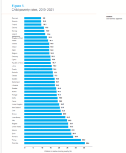
Source: UNICEF (2023, p. 11)
(iv) Material deprivation and other indicators of hardship
Official poverty measures, like those discussed above, can be supplemented with other indicators of hardship. An example of how material deprivation can be measured is Margaret Thomas’s 2022 study of US families. She analyses survey data that contains answers to questions about lack of money leading to hardship concerning: (i) food (received free food or meals during previous year?), (ii) housing (evicted, moved in with others, homeless at any time during previous year?), (iii) medical expenses (unable to afford medical care at any point during previous year?), (iv) utilities (cut off at any point during previous year?), and (v) bill paying (didn’t pay full amount of rent, mortgage, utility bill at some time during the previous year?).
Thomas’s data consists of five surveys representative of populations in large US cities. The surveys followed the same households from 1999-2001 until 2013-2015. She finds that bill-paying hardship is the most common, affecting from 30 to 35 percent of households annually. This was followed by utilities hardship (15 to 25 percent of households) and food hardship (around 10 percent of households). Medical hardship is the least common, affecting around 5 percent of households in any individual year.
Households vary from those typically having at most one type of hardship to those which typically have 2 to 4 types of hardship (2022, pp. 350-353). Thomas writes that “material hardship is a widespread experience among US families. In this study, about 40-50% of families experienced moderate or severe material hardship” in each survey. “60% of families experienced moderate, severe, or worsening longitudinal material hardship patterns” when considering all five surveys (2022, p. 360).
Other measures of hardship experienced by households are also available. To give just a couple of examples, in his book Poverty, By America, Matthew Desmond writes:
Between 1995 and 2018, the number of households receiving Supplemental Nutrition Assistance Program benefits (food stamps) but reporting no cash income increased from roughly 289,000 to 1.2 million, amounting to roughly one in fifty Americans. The number of homeless children, as reported by the nation’s public schools, rose from 794,617 in 2007 to 1.3 million in 2018. (2023c, p. 18).
Evidence like this contradicts the claim made in the Wall Street Journal article that Mankiw reprints which asserts that “War on Poverty is largely over and a success” (p. 406).
(v) Anti-poverty policy
Mankiw discusses the pros and cons of minimum-wage laws, cash payments (‘welfare’), a negative income tax (a kind of guaranteed minimum income), and in-kind transfers (pp. 409-413).
Mankiw doesn’t describe the reality of welfare payments. To start with, “[o]nly a quarter of families who qualify for Temporary Assistance for Needy Families [TANF] apply for it” (Desmond 2023c, p. 89). Then funds for TANF are paid by the federal government to individual states as a ‘block grant’. However, the states are not required to transfer those funds to needy families nor are they required to spend that money in each year. Matthew Desmond writes, “Nationwide, for every dollar budgeted for TANF in 2020, poor families directly received just 22 cents” (2023c, p. 28).
Supplemental Security Income (SSI), available in theory to sick and disabled people, is hard to receive in practice. Most applications are rejected; multiple applications are typically required, with many applicants having to hire a lawyer. Desmond estimates that about $39 billion of SSI benefits go unclaimed (2023c, pp. 31, 89).
Other programs also fail to deliver all eligible benefits. Federal housing assistance only reaches a quarter of the families who qualify for it (Desmond 2023c, p. 15). About 7 million people, eligible to receive the Earned Income Tax Credit (EITC), don’t claim it. Desmond estimates that $142 billion in aid annually goes unclaimed from the EITC, government health insurance, unemployment insurance and the SSI (2023, pp. 89-90). The likely causes: lack of information and/or the difficulties (perhaps intentionally constructed) in applying for benefits (2023c, pp. 122-123).
Thinking about a broad approach to anti-poverty policy, Desmond writes:
Poverty isn’t simply the condition of not having enough money. It’s the condition of not having enough choice and being taken advantage of because of that. When we ignore the role that exploitation plays in trapping people in poverty, we end up designing policy that is weak at best and ineffective at worst. (2023c, p. 78)
Let’s briefly consider some of the policies he advocates to deal with the exploitation of poor people in housing, labour and financial markets.
Housing. Vouchers to reduce rent costs; investment in public housing; assistance through loans to low-income families for homeownership (2023c, pp. 143- 149). De-concentrating poverty through inclusionary zoning to expand neighbourhood choice (2023c, pp. 161- 164).
Labour. Allow union organizing and bargaining to take place at the sectoral level as opposed to workplace by workplace; require worker representatives on corporate boards; increase in federal minimum wage (2023c, pp. 140-142).
Financial markets. Regulation of bank overdraft fees, payday lending. Increase the ability of low-income households to have and to access bank accounts and credit (2023c, pp. 149-150).
Beyond these, Desmond also argues for (among other things) improved reproductive choice (2023c, pp. 150- 155) and universal programs to help to “balance work and family life, programs such as paid family leave, affordable childcare, and universal pre-K” (2023c, p. 36).
To sum up: with the exception of the minimum wage, the anti-poverty policies discussed by Mankiw do not recognize or address market failures and power imbalances in markets that disproportionately affect low-income households. The policies advocated by Desmond do, while expanding freedom of choice.
- Wealth: Missing in Action
High and growing inequality of wealth in the United States has received considerable attention, both in the media and in high-profile economics research. Yet Mankiw chooses to ignore the subject entirely.
Wealth has an importance distinct from income. It’s possible to have a large income, but not to be wealthy in the sense of owning a lot of assets net of one’s debts. The distinction is often blurred in everyday language (and by Mankiw himself) when referring to high-income households as ‘rich’, when the dictionary definition of ‘rich’ is having a high level of wealth.
Being wealthy gives a household security and social status, among other advantages. It’s also obvious these days that being extremely wealthy – a multi-billionaire, for example – buys political influence in the United States.
This is not news to political scientists. In a well-known study based on a rare survey of the policy preferences of wealthy people, Martin Gilens and Benjamin Page concluded that “the preferences of the average American appear to have only a minuscule, near-zero, statistically non-significant impact upon public policy.” Instead, the preferences of the wealthy and of business interest groups dominate (2014, p. 575).
More than 90 percent of the expert panel, whose views on other subjects are quoted periodically in Mankiw’s text, agree or strongly agree that “the increasing share of income and wealth among the richest Americans is giving significantly more political power to the wealthy.”
Let’s briefly look at how wealth inequality has been increasing in the United States before looking at the distribution of wealth in more detail.
(i) The distribution and growing inequality of wealth in the United States
Figure 7 shows an estimate of the distribution of family wealth in the United States in 2022. Households in the first seven percentiles have negative wealth; their debts exceed their assets. Households in the 10th percentile have between $450 and $1000 in net worth.
Figure 7: Distribution of Family Wealth, 2022
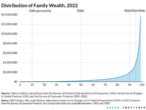
To be in the 50th percentile, households need a net worth between $192,700 and $201,830. Those in the 90th percentile have between $1,936,900 and $2,162,050. The 95th percentile has households with wealth between $3,795,600 and $4,694,300.
Membership in the top 1 percent – the 99th percentile – requires wealth above $13,615,400. This group includes the country’s billionaires, who number about 800 as of September 2024.
The Federal Reserve publishes quarterly estimates of the shares of total assets owned by different wealth percentile groups. It also has estimates of the shares of different asset types (e.g. real estate, corporate equities and mutual funds, private business, etc.). The following table shows some of these estimates.
Table 20.3: The Distribution of Wealth in the United States, 2024 (Q2)
| Wealth percentiles | Share of total assets | Share of corporate equities and mutual fund shares | Share of private business assets |
| Top 0.1% | 13.5 | 23.4 | 28.2 |
| 99%-99.9% | 16.7 | 26.4 | 24.7 |
| 90%-99% | 36.5 | 37.3 | 31.5 |
| 50%-90% | 30.8 | 11.9 | 14.6 |
| Bottom 50% | 2.5 | 1.0 | 1.1 |
Source: Distributional Financial Accounts, Federal Reserve.
According to these estimates, the top 0.1 percent own almost a quarter of the stock market and more than a quarter of private business. The top 1 percent own half the stock market and just over half of private businesses.
Inequality in the distribution of wealth in the United States in the 20th century has followed a U-shape. Saez and Zucman (2016, p. 519) write that “wealth concentration was high at the beginning of the twentieth century, fell from 1929 to 1978, and has continuously increased since then… The increase in wealth inequality in recent decades is due to an upsurge of top incomes combined with an increase in saving rate inequality.” The latter refers to the decline in the saving rate by the bottom 90 percent of income earners, so that, all else equal, their wealth increased more slowly, while those with high incomes accumulated wealth at a faster rate.
The result is a “snowball effect: wealth generates income, income that is easily saved at a high rate when capital taxes are low; this saving adds to the existing stock of wealth, which in turn generates more income, and so on” (Saez and Zucman 2019, p. 97).
Figure 8 shows estimates of the share of wealth owned by the top 1 percent from 1976 to 2024. During this time, the cumulative growth rate of wealth owned by the top 0.01% has exceeded that of the top 0.1%, which in turn has been greater than that of the top 1% as a whole. The share owned by the middle-class started to decline in the mid-1980s.
Figure 8: Wealth shares, 1976-2024
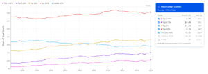
Source: realtimeinequality.org, accessed 5 January 2025.
(ii) Wealth inequality in the United States in international comparison
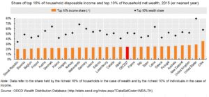
If wealth inequality is measured as the share of wealth held by the top 10 percent of the population, the United States has, by far, the greatest wealth inequality in the OECD. Figure 9 shows estimates for these shares for OECD countries and compares them with the share of income received by the top 10 percent of income recipients.
Figure 9: Top 10 percent of income and wealth shares, OECD
Source: OECD (2019, p. 99).
(iii) Reducing wealth inequality: wealth taxes
Emmanuel Saez and Gabriel Zucman (2019, p. 211 n. 18) write that in “the 1950s–1970s, wealth concentration was at a historically low level in America.” Growing wealth inequality since that time has led to wealth tax proposals.
Saez and Zucman offer a “radical wealth tax” proposal of their own as part of a package of tax reforms. In their view, growing wealth inequality due to accumulation at the very top “has not benefited the rest of the population – but has been chiefly at the expense of the working class” (p. 173). They claim that much of the increase in wealth at the top has been the result of rent-seeking activities – in other words, activities the transfer income from one group to another rather than generating new economic activity.
An annual wealth tax is needed because high marginal tax rates on very high incomes are not very effective in reducing wealth inequality. An increase in the value of a person’s assets is income, but taxable income includes only the gains realized when the assets are sold. If the assets aren’t sold, their accrued value can increase, increasing wealth; taxation is postponed until realization, should that occur. Most of the wealthy’s wealth consists of financial assets, including ownership of firms, that can be held a long time. As a result, even those with great wealth can report relatively little taxable income.
Saez and Zucman give the example of Warren Buffett (p. 129). His income in 2015 was at least $3.2 billion, measured on an accruals basis. Yet he paid federal income taxes of $1.8 million, for an effective tax rate of 0.055%. They explain that Buffett’s wealth
primarily consists of shares in his company Berkshire Hathaway. The company does not pay dividends. When it invests in other corporations, it forces them to stop paying dividends to. The consequences of this maneuvre? For decades, Buffett’s wealth has been accumulating, free of individual income taxes, within his firm… To finance any consumption needs, Buffett simply needs to sell a few shares.… He then pays tax – a modest one – on the small amount of capital gains he just realized. And that’s all.
Saez and Zucman’s radical wealth tax proposal: a marginal wealth tax rate of 2% above $50 million and 10% above $1 billion. The goal of the tax is not to make it harder to become a billionaire, but to “make it harder to remain a multibillionaire” (p. 174). They calculate that the tax would “de-concentrate wealth” in the long term.
Those whose wealth is growing very rapidly would continue to get richer, but eventually as they became ‘long-term billionaires’ like Bill Gates, their fortune would shrink. They write: “In the long run, a radical wealth tax erodes top fortunes so much that it reduces the taxes paid by the ultra-rich” (p. 175). The result would be a very significant reduction in wealth inequality.
REFERENCES
Brady, David (2021) American Poverty Should Be Measured Relative to the Prevailing Standards of Our Time, New York: The Century Foundation.
Desmond, Matthew (2023a) “America Is in a Disgrace Class of Its Own,” New York Times, March 16.
Desmond, Matthew (2023b) “Why Poverty Persists in America,” New York Times Magazine, March 9.
Desmond, Matthew (2023c) Poverty, by America, New York: Crown.
Geide-Stevenson, Doris and Alvaro La Parra-Perez (2024) “Consensus among economists 2020. A sharpening of the picture,” The Journal of Economic Education, 55(4): 461-478.
Gilens, Martin, and Benjamin Page (2014) “Testing theories of American politics: Elites, interest groups, and average citizens,” Perspectives on Politics, 12(3): 564–80.
Hill, Rod, and Tony Myatt (2022) The Microeconomics Anti-Textbook: A Critical Thinker’s Guide, second edition, London: Bloomsbury.
Lindert, Peter (2004a) Growing Public: Social Spending and Economic Growth since the Eighteenth Century, 2 vols, Cambridge: Cambridge University Press.
Lindert, Peter (2004b) “Social spending and economic growth. Interview with Peter Lindert,” Challenge, 47(4): 6–16.
Organization for Economic Cooperation and Development (2015) In It Together: Why Less Inequality Benefits All, Paris: OECD.
Organization for Economic Cooperation and Development (2024) Society at a Glance 2024: OECD Social Indicators. Paris: OECD.
Piketty, Thomas, Emmanuel Saez, and Stephanie Stancheva (2014) “Optimal Taxation of Top Labor Incomes: A Tale of Three Elasticities,” American Economic Journal: Economic Policy, 6(1): 230-271.
Ostry, J., P. Loungani and A. Berg (2019) Confronting Inequality: How Societies Can Choose Inclusive Growth, New York: Columbia University Press.
Saez, Emmanuel (2023) “Striking it Richer: The Evolution of Top Incomes in the United States (Updated with 2019-2021 estimates),” UC Berkeley Working Paper, 2023.
Saez, Emmanuel and Gabriel Zucman (2016) “Wealth Inequality in the United States since 1913: Evidence from Capitalized Income Tax Data,” Quarterly Journal of Economics, 131(2): 519–578.
Saez, Emmanuel and Gabriel Zucman (2019) The Triumph of Injustice: How the Rich Dodge Taxes the and How To Make Them Pay, New York: W. W. Norton.
Shrider, Emily A. (2024) Poverty in the United States: 2023, US Census Bureau, Current Population Reports, P60-283, U.S. Government Publishing Office, Washington, DC, September.
Thomas, Margaret M.C. (2022) “Longitudinal Patterns of Material Hardship Among US Families,” Social Indicators Research, 163: 341-70.
UNICEF Innocenti Global Office of Research and Foresight (2023) Innocenti Report Card 18: Child poverty in the midst of wealth, Florence: UNICEF Innocenti, December.
Urban Institute (2017). “Nine Charts about Wealth Inequality in America (Updated)”. Retrieved from https://apps.urban.org/features/wealth-inequality-charts/