Double deflation: Double Distilled or Double Dutch? Some remarks about the estimation of real economic production – Part 2
Download the WEA commentaries issue ›

Krzywy Domek, “crooked little house”.
This piece benefited from remarks by Stuart Birks, Josh Mason and Diane Coyle
In a previous article I explained one of the methods used by economists to estimate production and productivity: double deflation. This follow up article extends the argument, show how different estimation methods lead to differing results, pays some attention to institutional influences on prices and discusses how the problems mentioned here should influence the choice for policy variables like the inflation targets of central banks.
- Introduction: the anachronistic nature of productivity estimates
The double deflation method to estimate production and productivity is, according to the IMF, the method of choice for economists (Alexander e.a. 2017). According to the OECD, which also defends the use of this method, this method can lead to bizarre outcomes: “Another issue is the occasional occurrence of negative value added figures when double deflation operates with Laspeyres quantity indices. Nothing ensures that the subtraction of constant-price intermediate inputs from constant-price gross output yields a positive number” (OECD 2001, p. 45). If this happens, The OECD is clear on what to do: “In these circumstances different accounting method should be used to estimate an aggregate like value added, such as the methods based on “superlative” index numbers”. But maybe we should first try to understand why a ‘method of choice’ results in unpalatable outcomes. After all: even when value added is not negative it might still be wildly of the mark!
The first question is how a deflation method – i.e. a method which tries to disentangle changes in prices from changes in volumes – might result in negative ‘real’ value added. Value added is a nominal variable defined as the nominal value of production minus the nominal value of current inputs. The nominal value is influenced by changes in input and output prices as well as by changes in input and output volumes. Using the double deflation method to take the price changes out of the estimates of the value in inputs and outputs can, in specific historical circumstances, lead to a ‘volume’ index of inputs which rises much faster than the index of outputs while, at the same time, the value of inputs does, as input prices decrease relative to output prices, does not show such a pattern. An example: graph 1 shows the use of intermediate inputs in Dutch agriculture as a percentage of the value of output, measured in current prices as well as measured by using the double deflation method, i.e. using fixed prices.
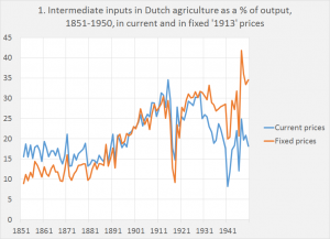
Looking at the historical of development of the use of intermediate inputs in Dutch agriculture (feed and fertilizer) it shows, after 1880, a rapid increase of the use of these inputs (the next paragraph is based upon Knibbe, 1993). This was caused by the fast increase of the use of (imported) feed after around 1880 and of (largely imported) chemical fertilizer after around 1895. Both developments were connected with an uptick in the rate of production growth as well as structural change. For one thing, farmers on the sand soils could dispense with the labor intensive practice of cutting card load after card load of heather sods, mixing these with sheep manure and spreading card load after card load of the resulting compost over them their arable lands. Instead of this, they could sell their sheep and buy some bags of chemical fertilizer and spread this quickly and efficiently over their lands, to obtain a better and more secure harvest with much less toil. Within decades, the hundred years old practice of cutting heather sods was abandoned, aided and facilitated by railroads which transported the fertilizer, government extension and research services which taught farmers how to use fertilizer and which investigated how much was needed and agricultural cooperatives which broke cartels of fertilizer producers. As a result, use of monetized intermediate inputs, measured as a percentage of output, rose dramatically – but use of own produced intermediate inputs declined.1
The increased use of purchased inputs of course had a catch. Farmers became more dependent on the market which meant that a disruptions of the market (the world wars come to mind) could wreak havoc with this kind of input intensive farming while a poor local harvest might leave them indebted to suppliers. But there is more to this story. After 1929 the value of intermediate outputs used, measured as a percentage of current output, declined dramatically while intermediate outputs, measured using the double deflation method, stayed level. Thanks to lower prices for feed and fertilizer (and government policies which increased the prices of outputs) relative prices of inputs compared with prices of outputs declined, which explains the diverging trends of the two series. Looking more closely at the graph teaches us that a comparable development took place around 1880, when cheap imports of feed became available
As far as I’m concerned, the differing developments of the two lines point out an extremely important development: a decline of prices of intermediate inputs relative to outputs which was pivotal to a profound transformation of farming and agriculture – and also to a profound change in the distribution of total income generated in farming.2 Developments which are missed when we only look at ‘volume’ estimates, even if these volume estimates of production were unproblematic. But what does it mean for our estimates of productivity? Nominal value added can be understood as an estimate of production, but also as an estimate of income. In the latter case, deflating value added with an index of the consumer prices is the apt procedure to calculate a ‘real’ variable, in this case purchasing power (one has to use net value added here, not gross value added). This makes sense. But was does subtracting an index of the use of intermediate inputs from an index of the use of outputs in fact mean? Using more natural gas to heat an office building during a cold winter will diminish nominal value added as well as double deflated value added – but does it also decrease production and productivity of the office workers? The concept of double deflated value added is not entirely straightforward.
A comparable argument is made by Edquist (2013). According to him the extremely high growth rate of productivity in Swedish production of electronics (40% a year…) is due to subtle biases of the double deflation method (Edquist, 2013). Swedish manufacturing of electronics is dominated by one company, Ericsson. Large Ericsson losses in one year led to (almost) negative nominal value added for this company. The subsequent large increases in value added showed up as extreme increases in productivity; just looking at the double deflated data only conflates the situation instead of illuminating it. In his words: “when productivity is analyzed for these types of industries it is important to base the analysis on both value added and gross output to test the robustness of the results” (Edquist, 2013, p. 9). Also, recently Peter Lindert used a related argument in his contribution to the discussion about the question if ‘the West’ surged ahead of the rest of the world already in the seventeenth and eighteenth century (Lindert 2017). Instead of using anachronistic 1990 prices of inputs and outputs to compare the relative level of prosperity in centuries past, a more direct approach may be advisable: “It is far easier, and more appropriate to historical contexts, to stick with direct current-price comparisons of the countries’ nominal incomes per capita back then, deflated by prices people paid back then.” Doing this made a difference. For one thing, western dominance was not just a question of western growth. But also of non-western stagnation and decline, exemplified (according to the data of Lindert) by the long run development of the Dutch colony of Java. While India was already very poor to begin with (1595). Again, the choice of prices and methods to measure historical processes clearly matters. On the most basic level, this is caused by the fact that we are living in a monetary world – and (relative) money prices matter. Value added is a fundamental monetary variable. It surely enhances our understanding to investigate how changes in productivity influence value added. But in a monetary world, productivity can never be understood from changes in market ‘volumes’ alone. Production functions are inherently monetary and prices are a function of the institutional surrounding. As a consequence, volume estimates, useful as they are, can only be understood in context. Volume estimates of production and productivity can be quite misleading when understood in their own terms and even unpalatable, according to the SNA 1993 (quoted in OECD 2001): “a process of production which is efficient at one set of prices, may not be very efficient at another set of relative prices. If the other set of prices is very different, the inefficiency of the process may reveal itself in a very conspicuous form, namely negative value added”. And it’s up to the economist to investigate what these inefficiencies are and why they arose, surely when we consider that even when double deflated value added is not outright negative it might still be far of the mark.
- Adding an insult. Index number theory
Such problems arise because productivity, as economists define it, is not something physical like wheat per hectare, phone calls per call centre employee, spectators watching a particular football game or the occupancy rate of hotels or planes. But a monetary phenomenon: economists estimate value added per hour of labor or unit of capital.3 Above, we’ve seen that the OECD advises to use “superlative’ index numbers to avoid the problems which one can encounter when using the double deflation method. “Superlative” methods enable one to estimate a price or volume series which uses a new base year every year, which prevents the problem of using anachronistic prices of a fixed base year which becomes less relevant with every year that passes. Even then, arithmetical quirks (related to ever changing weights of these methods) can lead to less palatable outcomes. Graph 2 compares two price indexes of Dutch arable production (which I took as I have the data but also, and more important, because arable products do not change too much).
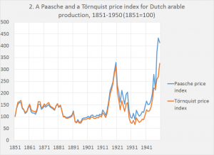
One consists of spliced Paasche indexes with a fixed based year which were calculated for a number of sub periods. The other is a superlative Törnquist index, which is rebased every year. As can be seen, the long run development of the indices is quite different. Somehow, price declines must have gotten a relative larger weight or price increases must have gotten a larger weight, compared with the Paasche index. Using one of the Irving Fisher tests of price indexes (the increase of the index should lie between the price increases of the goods and/or services with the lowest and the highest price increase) shows that the Törnquist index only barely survives this test. Only one product (wheat) has a price increase which is lower than the increase of the aggregate Törnquist index (295 vs. 326). The theoretically less ideal Paasche index is as such more plausible as it is near the median as well as the arithmetical average of price changes (8 products have a larger increase, 4 products have a lower increase). Economic statisticians are of course well aware of this and other problems and in reality use, next to the double deflation method, a plethora of methods, maybe not all of them theoretically sound, to produce volume estimates of value added (Eurostat 2015, especially figure 5). Which reminds us of the suggestion of Edquist, cited above. Using one method only to calculate production and productivity might just not be the answer.
3.What to do?
Estimating ‘real’ economic growth is a noble and worthwhile pursuit. But economists should take heed that value added is, fundamentally, a nominal variable. Deflating it will, among other problems, lead to all the well-known problems related to the use of deflators for constructing time series: there is no ‘right’ way to disentangle price increases from changes in relative prices. Double deflation does not only doubles that risk and adds the possibility that unpalatable magnitudes of ‘real’ value added are calculated, which obfuscate instead of enlighten.
Instead of this – or better: next to this – economists would do well to focus on these intermediate inputs which are subtracted from output and do not seem to have an independent role in increasing value added – at least not in neoclassical growth accounting. We’re talking among other things about energy, water and the like. Fortunately, we do have existing estimates of real ‘real’ use of inputs – i.e. information in tons and gigawatts – which are largely based upon the same national accounts as the value added series. Eurostat, 2016, calculates use of material resources and production of CO2 related to final use (consumption, investment, net exports), which shows that post 2008 housing bust led to a sharp decrease of the use of materials. A recent flagship UN report written by the International resource panel and titled ‘resource efficiency: potential and economic implications’ (International resource panel, 2017) contains extensive data on use of a whole array of resources, like different materials, land, water and energy and how these are used. And uses among other metrics ‘material footprints’ as variables to estimate productivity. Instead of subtracting inputs it surely is worthwhile to look at how these actually contribute to productivity. Tracking such more technical variables and using input-output tables to do this might enhance our understanding of why real production increased. The value added estimates, broken down in constituent parts like wages, profits, rents and interest can subsequently teach us how the spoils are distributed.
Literature
OECD (2001). Measuring Productivity. OECD Manual Measurement of aggregate and industry-level productivity growth. Paris: OECD. Available here.
Agrawal, Raj; Büttgenbach, Thomas; Findley, Findley, Jeddy, Aly Jeddy, Petry, Markus; Kondo, James; Lewis, Bill; Subramanian, Guhan; Borsch-Supan, Axel; Huang, Kathryn; Greene, Seane et al (1996). Capital productivity. Washington: McKinsey Global Institute.
Edquist, Harald (2013). “Did Double Deflation Create the Swedish Manufacturing Growth Miracle? Is There a Lesson for Other Western European Countries and the US?”. Economics letters 121-2 pp. 303-305. Available here.
Eurostat (3 November 2015). Building the System of National Accounts – volume measures. Retrieved 19 April 2017. Available here.
Eurostat (March 2016). Carbon dioxide emissions from final use of products. Retrieved 20 April 2017. Available here.
International resource panel (2017). Resource efficiency: potantial and economi implications. New York: United Nations environment program.
Knibbe, Merijn (1993). Agriculture in the Netherlands 1851-1950. Production and institutional change. Amsterdam: NEHA
Lindert, Peter (17 April 2017). “European and Asian incomes in 1914: New take on the Great Divergence.” Voxeu, available here
- The series actually consists of a number of spliced sub series, each with their own base year set of prices, to take account of changes in relative prices. I used this particular series because I had the data but also because agricultural products do not change too much over time, which means that all kinds of problems connected to quality changes of products do not raise their head.
- For the history nerds: the fast mechanization of Dutch agriculture would only start after about 1955.
- Estimates of the magnitude of the ‘volume’ of the aggregate value of capital suffer from the same problem. A fascinating example of this is Agrawal e.a. (1996), a McKinsey Global Institute flagship publication with an advisory committee consisting of no less than Bob Solow, Ben Friedman, Zvi Griliches and Ted Hall, at the the cream of the crop when it came to estimates of capital. While the authors consistently write about physical capital the text shows that they use the national accounts estimates of capital, which are aggregates of the monetary value of capital beset with the same kind of relative price quirks (even more so, in fact) as estimates of production or inputs. The authors do not seem to be aware of this; a welcome addition to neoclassical growth theory, which only takes account of produced capital is however that, as they use national accounts data, information on ‘land’ (i.e. non produced capital) are included.
An additional note on double deflation
“All of these measures are carefully developed but have their own limitations. Those who use the data we produce should recognize these limitations and exercise judgment accordingly concerning whether and how the data ought to be used”
Abraham and Moulton, quoted in Perry (2014)
Double deflation is constructing time series of weighted averages of outputs (wheat, sugarbeet, whatever) as well as a weighted average of inputs (fertilizer, energy, pesticides, whatever) and subtracting outputs from inputs. Prices of outputs and inputs are used as weights. This seems straightforward, as value added (the amount of money available to pay wages, rents and ‘mixed income’ of a farmer or small businessman or –woman) is also equal to the value of outputs minus the value of inputs.
There is however a catch. Relative prices change. Suppose that energy prices increase while all other prices stay equal. Nominal value added will decrease and, as ‘mixed income’ is risk bearing, mixed income will decline. Using fixed prices from before the rise of oil prices won’t show this: ‘real’ value added, as it is called, will stay equal or, when volumes of inputs or outputs change, only change because of these volume changes. Which leads to the question: which set of ‘fixed’ prices will be used to calculate ‘real’ value added? Of course, one can change this set of fixed prices every year, calculate growth rates between two years and splice all these growth rates. To calculate growth between 2014 and 2015, 2014 prices are used. To calculate growth between 2015 and 2016, 2015 growth rates are used. And the growth rates are spliced. This is what statisticians mean with ‘chain weighted indexes’. This has, however, some problems. It is very well possible that a sector grows faster than the entire economy but that prices in this sector decrease. ‘Real’ value added will show an increase but nominal value added will show a smaller increase, relative to the rest of the economy of, as happens on a regular basis in the real world, even a decrease (a case in point: shale oil during the first months of the abrupt decline of oil prices between October 2014 and January 2015).
Also, and more important: what does {‘real’ output – ‘real’ input} actually mean? Nominal output minus nominal input is, to me, a clear concept: the amount of money available for incomes (or, when measured on a gross basis, also for replacement investments). And (net) nominal value added divided by a consumer price index is equal (or at least a good approximation) of the purchasing power of nominal value added. But I have difficulty grasping the meaning of series of ‘real’ output minus ‘real’ input. One can of course relate the use of inputs (feed, fertilizer, manure) to the production of outputs (Knibbe, 2000). One can also investigate the influence of availability of real products on prosperity (for food: Knibbe, 2006). These analyses are based upon national accounts estimates. These accounts force the researcher to construct complete and coherent estimates of inputs and outputs which, next to estimates of nominal output, for the very reason of their coherence and completeness, can be used to investigate productivity or prosperity looking at actual inputs or outputs. But ‘double deflation’ only seems to make sense in a one product economy, where coconuts are either consumed or used to grow new coconuts. Which leads us to critiques of this kind of ‘one product’ thinking. In the words of Marx (ht: Josh Mason): “we have the complete mystification of the capitalist mode of production, the conversion of social relations into things (i.e. coconuts, M.K.), the direct coalescence of the material production relations with their historical and social relation. It’s an perverted, enchanted, Topsy-turvy world in which Monsieur le capital and Madam la Terre do their ghostwalking as social characters and in the same time directly as mere things”. Marx did not write about double deflation but reducing output and input to a one product economy without social relations fits into such kinds of critiques. The whole Schumpeterian development hinted at in the main text is left out of the analysis and the distribution of nominal value added (who owns the land) is rendered impossible as the ‘real’ variable measured is thus opaque that it disables any meaningful analysis of distribution (at least at the sectoral level). Those inclined to dismiss such critiques by stating that price indexes are technocratic entities are advised to read Rippy (2014): economic indicators are always forged in a political fire. Chain weighted indexes do enable Schumpeterian analysis if only by investigating how and why weights changed but this does not happen too much.
Aside from this price and volume indexes have their technical problems. In a very useful oversight Diewert (1992) lists 21 ‘reasonable’ tests indexes have to satisfy – and many frequently used indexes do not satisfy quite a lot of these (Diewert is in favour of the Fisher index); Diewert however refrains from stating how indexes can be used in dynamic economic analysis.
Literature
Diewert, Walter (1992). “Fisher Ideal Output, Input and Productivity Indexes Revisited”, Journal of Productivity Analysis 3-3 pp. 211-248
Knibbe, Merijn (2000). “Feed, fertilizer and agricultural productivity”, Agricultural history 74-1 pp. 39-57.
Knibbe, Merijn (2007). “De hoofdelijke beschikbaarheid van voedsel en de levensstandaard in Nederland 1813-1950 (The per capita availability of food and the standard of living in the Netherlands, 1807-1950)”, Tijdschrift voor sociale en economische geschiedenis 4-4 pp 71-107
Rippen, Darry (2014). “The first hundred years of the Consumer Price Index: a methodological and political history“, Monthly Labor Review, U.S. Bureau of Labor Statistics
From: pp.8-12 of WEA Commentaries 7(2), April 2017
http://www.worldeconomicsassociation.org/files/Issue7-2.pdf