Birks – Mankiw 7th edn Chapter 33: Aggregate Demand and Aggregate Supply
Mankiw, N. G. (2015) Principles of economics (7th ed.) Ch.33
Principles of macroeconomics (7th ed.) Ch.20
Mason, OH: South-Western Cengage Learning
Aggregate Demand and Aggregate Supply
When reading the chapter, here are some aspects to consider:
1. So far Mankiw has been looking at the economy in the long run. This chapter takes a short run perspective considering “short-run deviations from long-run trends”. There is a particular framing in this, suggesting that the long run and the short run can be considered separately. An alternative view would be to consider short-run events as having an impact on outcomes in the long run, as might occur with “path-dependence”. Mankiw’s Figure 1(a) seems more like a disrupted growth path, with an upward climb interrupted by periods of slowdown in the recessions. These come across as rightward shifts in the curve, or a series of “steps”, rather than deviations around a trend line. There can be lost investment and disrupted employment patterns in a recession, and these have implications for future potential GDP.
2. Recessions are defined in NZ (and elsewhere, including the UK) as two successive quarters of negative GDP growth. The US relies on decisions by the Business Cycle Dating Committee of the National Bureau of Economic Research (NBER). Depressions are severe recessions, one rule of thumb being a decline in GDP of at least 10%.
3. For the shape of the Aggregate Demand Curve, note the components – these are standard. In Mankiw’s simplified representation, there is a separate effect for each of variables C, I and NX. This makes the analysis easy, but may be oversimplified. Note that G is exogenous, or determined outside the system. Variables whose values are set within the specified system (or model), are referred to as endogenous.
4. At all points on the AD curve, Y = C + I + G + NX
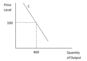
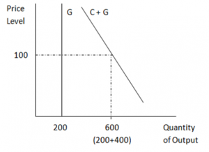
As the components on the right are summed to give the final curve, we could consider them as individual curves giving the amount of each as the price level varies. Adding them up is a similar process to the horizontal summation of individual demand curves to construct i) a market demand curve, or ii) private plus public saving to get a savings curve, or iii) domestic investment (I) plus NCO to get a demand for loanable funds curve (as in Chapter 32). Mankiw then discusses the determinants of each of these components. First, he considers how they each relate to the price level, with this operating through a different mechanism for each of C, I and NX:
- C is a function of the price level via the wealth effect.
- I is a function of the price level indirectly via the effect of price level on the interest rate
- NX is a function of the price level indirectly via the effect of price level on the interest rate and subsequently on the exchange rate.
These are assumptions in his model and may bear little similarity to the real world. For each of these relationships, a lower price level is assumed to result in higher expenditure.
G is assumed to be exogenous (determined outside the model), and so does not vary as the price level changes. This means that G would be a vertical line. We can plot these as follows, just using C and G to illustrate:
5. Mankiw gives an ad hoc explanation of the Aggregate Demand Curve. A more involved alternative is to use the Keynesian Cross model (discussed in points 7 and 8 of this commentary to Chapter 26). This model considers the determination of an equilibrium income at some specified price level. (Note that, in that model, the 45-degree diagram gives the level of expenditure on the vertical axis and income on the horizontal axis. Consequently the components of expenditure are summed vertically and government expenditure, being independent of income, is a horizontal line.) We can find the equilibrium in that model for different price levels, thus getting a series of points on the AD curve. In other words, the AD curve can be thought of as showing the relationship between equilibrium GDP and the price level (as determined by the Keynesian cross model). Changes in variables in the model other than the price level can then result in shifts of the curve. Derived in this way, it is clear that the AD curve is not equivalent to a microeconomic demand curve.
6. Mankiw’s derivation of the long-run Aggregate Supply Curve now gives a graphical representation of the assumption made for the textbook material up to now, namely that the economy is at long-run full employment and the at “natural rate of output”. He then gives an explanation as to why the relationship may be different in the short run.
7. Note the general idea of a variable, Y, being a function of several other variables (and identify what these are where necessary). Then recall the standard relationship with a graph of say Y against X. Changes in X can result in a movement along the curve, whereas changes in any of the other variables can result in shifts of the curve.
8. A final word of warning. The AD-AS model is not a demand and supply model such as Mankiw’s Chapter 4. AD can be seen as plotting a series of equilibria in one part of the economy (income and expenditure). The AS curve plots a series of equilibria in another part (production decisions). Where they meet, both parts are in equilibrium, so there is no incentive for participants in either part to change their behaviour. There may still be disequilibrium elsewhere, such as in labour or financial markets. Changes there may then impact on AD and/or AS. In other words, we can gradually build up a more complex structure, bringing more variables into the overall model, changing them from exogenous to endogenous.
Commentary by Stuart Birks, 5 September 2014

